Quick Analysis Tool in Excel: Everything You Need to Know
Microsoft Excel works wonders in data analysis and visualizations through its many formulas, functions, features, elements, and graphs. Did you know that the application can also assist you with or suggest options that help you in slicing and dicing data?
You heard it right! Quick Analysis tool in Excel is one such functionality that single-handedly caters to all sorts of data analysis and visualization works. Read on to learn all you need to know about the Microsoft Excel Quick Analysis tool.

What Is the Quick Analysis Tool in Excel?
The Quick Analysis tool (QAT) is simply an aggregation of various popular data analysis tools of Excel in one easily available context menu.
While you need to make many mouse clicks to create a graph, table, Pivot table, or summation, the Quick Analysis tool lets you do all these in a single click.
Microsoft introduced this feature in Excel 2013, and since then, all the latest versions of Excel come with the Quick Analysis tool by default.
The functions and commands of the Quick Analysis tool are fixed. Also, depending on the data range that you’ve selected, Excel would show personalized functions through the tool.
For example, if the selected cell range doesn’t contain more than three columns of data you won’t see the Pivot table option in the Quick Analysis toolbox. Similar to the data range, it also understands the type of data that you select, like numbers, currency, dates, texts, months, etc.
How to Locate the Quick Analysis Tool in Excel
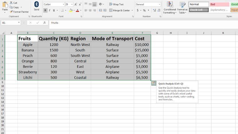
Excel’s Quick Analysis tool should always be available in Excel 2013 and new software unless someone has turned it off. More on that later. To use the QAT, simply select a range of cells. While keeping the cells selected look at the bottom right corner of the selection area.
You’ll find a small and interactive icon. Click on that icon to find the suggested data structuring, analyzing, graphing, and formatting tools in Excel for the selected cell range. Alternatively, select a single cell within the data and hit Ctrl+Q to instantly launch QAT.
How to Activate the Quick Analysis Tool in Excel
If you’re using Excel 2013 or later and yet the Quick Analysis tool is missing, try these steps to activate this cool functionality in your Excel app:
- Open the Excel workbook in question.
- Click on the File menu located on the Excel ribbon menu.
- Now, select Options from the left-side navigation pane.
- The Excel Options dialog box will open. It also has a left-side navigation pane with a few selectable menus.
- Choose the General menu.
- At the right-side pane under the User Interface options, you should find Show Quick Analysis options on selection.
- Select the check mark beside it and click Ok to save the settings.
Quick Analysis Tool in Excel: Functions
Depending on the data you select, you’ll find the following commands in Excel QAT:
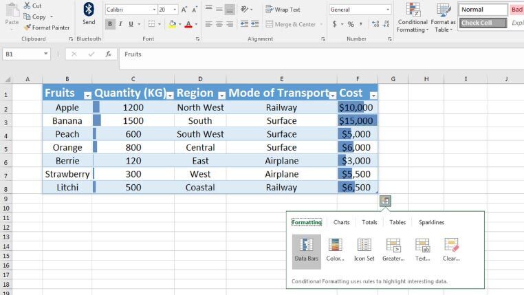
- Conditional formatting like Data Bars, Icon Sets, etc., to highlight interesting data.
- Charts like Clustered Bar graphs, Nested Bar graphs, etc., for data visualization.
- Automatic calculation of Totals like Sum, Average, Count, % Total, etc.
- Tables and Pivot tables to summarize, filter, and sort data.
- Sparkline-type mini charts to make dashboards look professional.
Final Words
So far, our in-depth discussion should have helped you determine precisely what the Quick Analysis tool in Excel is. You have also learned about select Excel functions and commands of the Quick Analysis tool and how to use them during your data analytics work.
If you love to learn new things about Excel you’ll definitely find this article interesting: Add Leading Zeros in Excel.