How to Alphabetize in Google Sheets: Know the 4 Best Methods
Google Sheets offer some excellent tools for working with data and discovering actionable insight. One such tool is organizing column data alphabetically.
But, you may be wondering how to alphabetize in Google Sheets? Your search ends here! Continue reading to learn the best methods of alphabetizing data ranges or the entire worksheet.

How to Alphabetize in Google Sheets
1. Using the SORT Function: Single Column
If you need to quickly alphabetize a range of cells in a column of data, the SORT function is the best choice. Try these steps for instant sorting:
- Ensure there are some data in a column of the worksheet.
- Select any cell where you want the alphabetized data.
- We’re going to sort data from column A (cell range A2:A26) to column E (cell E2).
- The formula will also work if you choose another source cell range and a target cell.
- In the target cell, copy-paste the following formula:
=SORT(A2:A26)
- The first name of the customers will show up in alphabetical order.
2. Using the SORT Function: Multiple Columns
When you need to alphabetize more than one column of data, the SORT function includes additional arguments. For example, you need to mention the sort column against which you want Google Sheets to sort your data.
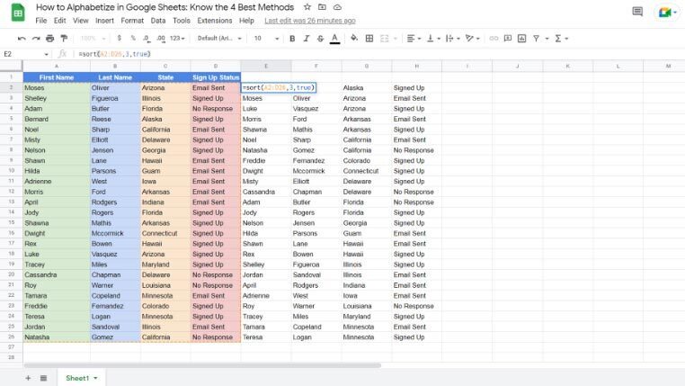
If you want to sort against column A, enter 1, for column B, enter 2, and so on. You also need to put ascending sort order by entering TRUE or FALSE. Try these steps to see for yourself:
- Go to the target cell and enter the following formula:
=SORT(A2:D26, 3, TRUE)
- You need to change the cell range address according to the data.
- Hit Enter.
- Google Sheets will alphabetize the data against column 3, which is C (State).
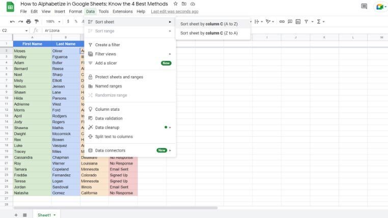
3. Using the Sort Sheet Tool
The Sort sheet tool lets you alphabetize all the sheet data in several columns against columns A, B, C, etc. You can choose between Z to A or A to Z sort order. If your worksheet data contains column headers, you need to freeze those headers as well. Here are the easy steps to try:
- Select the first cell of the header row and click on View.
- Now, hover the cursor over Freeze and then select 1 row.
- Select any cell under columns A, B, C, and D, or any other column on your own worksheet.
- The sorting tool will sort data against the selected column.
- Now, click on Data and hover the cursor over the Sort sheet.
- Choose the option Sort sheet by column C (A to Z).
- Google Sheets will automatically alphabetize all data.
4. Using the Advanced Range Sorting Options
When you select a cell range and go to Data and hover the cursor on Sort range, you’ll find the Advanced range sorting options. You may use this tool to sort multiple cell ranges depending on each other.
When you’re using this tool, you don’t need to freeze the header row. Simply check mark the Data has a header row option.
Conclusion
The above methods are the answer to your search for how to alphabetize in Google Sheets. You can use the formula-based approach when you need dynamic alphabetizing. Alternatively, go for a built-in sorting tool for the simple and automatic organization of cell ranges alphabetically.
You may also want to learn how to add drop down list in Google Sheets to make data entry work error-free, convenient, and organized.