COUNTIF Function In Excel 2010
In Excel 2010 by using COUNTIF conditional logic, you will be able to count occurrence of data and show the result if the condition is met. It enables user to use a condition that contain two arguments (range,criteria), that would be applied on data which yields counting results, only if specified criteria is TRUE. Thus facilitating user to create a group for certain type of data that falls into specific category. This post explains simple usage of COUNTIF logic.
Launch Excel 2010, and open a datasheet on which you need to apply formula with COUNTIF function.
For Instance: We will use student grading datasheet, containing student records.
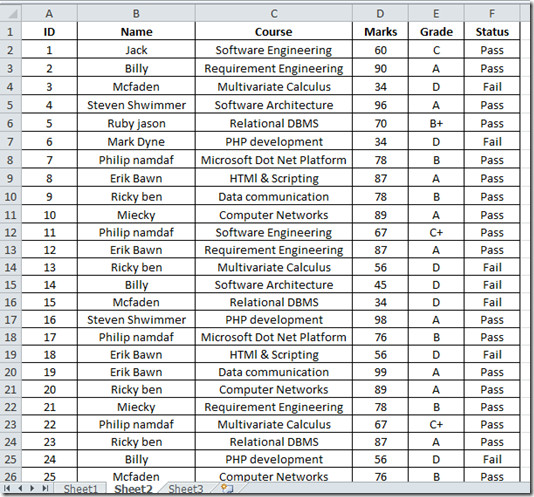
Now for checking how many students have secured A, B+, B, C+, C grade and how many failed in exam.
Here our primary concern is with Grade field, we will write a formula that will check the Grade column and count, how many students secured same grades.
Syntax:
=COUNTIF(range, criteria)
Now we apply formula complying with the syntax.
=COUNTIF(E2:E26,"A")
E2:E26 in the formula will select column E starting with row 2, to the end of the column E26. on selected column, a condition is applied that counts how many students secured A grade. This formula shows that 9 students secured A grade.
![table 2[2]](https://www.addictivetips.com/app/uploads/2010/04/table22.jpg)
Now we will create all other categories by changing the conditions that match with corresponding grades.
B+ Grade Students
=COUNTIF(E2:E26,"B+")
B Grade Students
=COUNTIF(E2:E26,"B")
C+ Grade Students
=COUNTIF(E2:E26,"C+")
C Grade Students
=COUNTIF(E2:E26,"C")
Fail Students (D grade)
=COUNTIF(E2:E26,"D")
The final Grading datasheet is shown in the screenshot below.
![table 3[3]](https://www.addictivetips.com/app/uploads/2010/04/table33.jpg)
You can also checkout previously reviewed SUMIF Function in Excel 2010.

may anyone please tell me about the formula if I wanna get the subject in which a student is fail. If there are 5 subjects and if any student is fail in any one or two, is it possible that the subject in which the student is fail that subject may display like fail in science & english
Can you use 1 COUNTIF function to search for A’s or B+’s? Or do you need to write it as a count of the A’s plus a count of the B+’s?
I tried the same step but the result I got were all “0”, any idea why?
The only thing you have to do is update the range of L7:L49 depending on which row and columns your letter grades are stored in.
=COUNTIF(L7:L49,”A*”)&TEXT(A1,”Ꭺ▬# “)&COUNTIF(L7:L49,”B*”)&TEXT(A1,”Ᏼ▬# “)&COUNTIF(L7:L49,”C*”)&TEXT(A1,”Ꮯ▬# “)&COUNTIF(L7:L49,”D*”)&TEXT(A1,”Ꭰ▬# “)&COUNTIF(L7:L49,”TC”)&TEXT(A1,”ʨ# “)
Well since nobody on the Internet has found a way to do this COUNTIF by providing results into a single formula with output to a single cell I wanted to share.
NOTE:
1) To make this work using the &TEXT option you must ensure cell A1 is blank of all data.
2) Since TEXT was not original designed in quite this way the text in “use special characters” from Adobe Latin Character Set from Windows Character Map. If you replace them with standard characters your formula will display as #VALUE indicating an error so paste from the text below to ensure best results–make sure your cell is wide enough for display.
3) Since I only wanted to total letter Grades of A, B, C & D and University Transfer Credits not part of the GPA calculation (Example Prior Learning Recognition) I included a Latin TC. If you do not require this you may change the last COUNTIF ,”TC” to “F*” using regular characters then replace the final ʨ special character with a Latin F.
=COUNTIF(L7:L49,”A*”)&TEXT(A1,”Ꭺ▬# “)&COUNTIF(L7:L49,”B*”)&TEXT(A1,”Ᏼ▬# “)&COUNTIF(L7:L49,”C*”)&TEXT(A1,”Ꮯ▬# “)&COUNTIF(L7:L49,”D*”)&TEXT(A1,”Ꭰ▬# “)&COUNTIF(L7:L49,”TC”)&TEXT(A1,”ʨ# “)
i tried to include &COUNTIF(L7:L49,”E*”)&TEXT(A1,”E▬# “) but got #Value instead. Please help. Thank you.
Hi Jake, just copy the following formula. However, do note that you need to change the “Range” (D6:L6) part to suit your worksheet.
=COUNTIF(D6:L6,”A*”)&TEXT(0,”A# “)&COUNTIF(D6:L6,”B*”)&TEXT(0,”Ᏼ# “)&COUNTIF(D6:L6,”C*”)&TEXT(0,”C# “)&COUNTIF(D6:L6,”D*”)&TEXT(0,”Ꭰ# “)&COUNTIF(D6:L6,”E*”)&TEXT(0,”Ε# “)&COUNTIF(D6:L6,”F*”)&TEXT(0,”F#”)
Hope this works.
Can I apply to countif to a filtered column and have it count just the cells in view ( not the ones hidden by the filter)- at the moment even if a column of 100 cells is reduced to 40 (say) the countif still counts all 100
Is there a way to combine 2 CountIf functions, for example, count all that equal 96 and A? That would not be useful in this example of course, because all 96’s would by default be A’s. But for what I am attempting, it would be useful.
HI,
you can try with IFwith AND and count the respective data by using COUNTIF.
=IF(AND(C2=96,B2=”A”),1,2) and apply COUNTIF for calculating 1.
How would you count a grade that is an A*. I have tried “A*” but that counts all the A and A*. I need just the A*.
Thanks
Use a ~ ahead of the * character in the formula … =countif(A1:A12, “A~*”)
I am facing a shocking result of the countif function.
=COUNTIF(A2:A300,”Amazon”)
gives a wrong result of counting.
like if actual is 28, its shows 29
always 1 extra to the actual.
Anyone know whats going on???
Regards,
Please explain how to use vlookup and count if please briefly explain
Md Afsar
Would you be able to help me out with a query on how to create a condition that will identify in addition to identifing how many grade As bs etc, but also identifying the Lowest grade A mark, grade B mark and grade C mark?
ive tried combining the COUNTIF statment with a MIN statement but so far unsuccesful.
Any help would be greatly appreciated.
Adam
This shouldn’t work. As an “A” grade is over 80, when the countif function goes to count “B” grades it will count all grades in the range over 75. An “A” grade is over 75 and will get counted with the “B” grades.
Thanks for pointing it out. We have updated the guide.
sir, if there is gape b/w range, eg in attendance sheet there is sunday then how we will range the attendance of this sheet?