Excel 2010: Freeze Rows And Columns
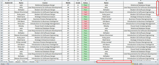
Excel 2010 comes with Freeze Row and Freeze Column features, which make it easy to match and read details of huge data sets. If you are dealing with huge datasheet containing student records, then you may want to freeze top row or first column to easily understand data while scrolling up / across the datasheet. In this post, we will take a look at how to freeze top row and first column.
In order to make the first column and row label apparent while scrolling, you need to follow very simple steps.
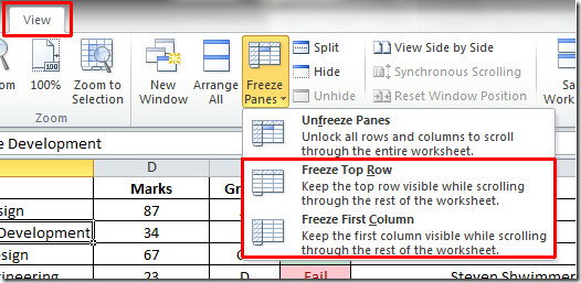
First off, head over to View tab, click Freeze Top Row to make the row labels appear, when you are scrolling.
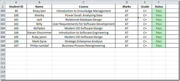
As shown in the screenshot below, top row labels are visible even at the bottom of the page.
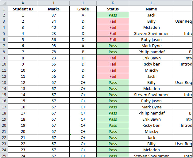
Now if you want to freeze first column, Click Freeze First Column, to do the same with the columns.

My header is composed on many rows. How do I freeze not one but two or three top rows?
I would like to freeze column A,B & C. How do I freeze all three?
Hi, it might be too late but the trick is very simple: Click a single cell and then click “freeze pane”. Any row above your selected cell and any column on the left of your selected cell will be frozen. For example click on B5 and then “freeze pane”. Your column A and rows 1-4 will be frozen.
The solution given by Baselben about dragging your cursor worked for me – thanks for saving me all the frustration I had been experiencing! And to CD. I would say that the tab furthest right in my Excel 2010 is “view”!
Can I freeze both the top row and the first column? I have been trying to do that for the last 2 hours but I when I freeze the top row and go to freeze the first column it unfreezes the top row! Frustrated
Could I Freeze column one and Row one….?
Yes, you can. Put the Cursor on B2 and go to VIEW; FREEZE PANES ( you have to unfreeze Panes if that option is not available and then FREEZE PANES) and save file. It works! 🙂
I was able to freeze the top row and the first 4 columns. Click the cell to the lower right of the area to be protected then click on Freeze Panes under View. i.e. To freeze row 1 and columns A, B, C, D then click on E2 followed by “Freeze Panes”
thanks so much!
to freeze any row, that is
Is it possible to any row? The only options I see are top row, first column, and unfreeze. I need to keep the first column frozen as is
just forget about micro$hit and use openoffice!
I agree but my company forces ms on us. And 2010 is not intuitive.
Is there a way to make the changes permanent? Also, can you freeze the first row and first column at the same time?
Click on the link bellow, It will solve 2nd part of your problem
http://www.techonthenet.com/excel/questions/freeze2_2010.php
i want to freeze in excel 2010 how i do it pls suggest me
“details could very tedious work to uncrude”…. your grammar truly sucks.
Please help: I want to free the first four columns in Microsoft Excel 2010
how do i freeze 5 consecutive rows
Select 6 consecutive rows and click on the Freeze Panes in View Tab
my excel have no view icon… pls help…
See Mike’s comment below. I got it to work (freezing top two rows) by choosing “Split” and then dragging the split bar down to where I wanted it (after row 2, not row 1). That worked!
How come you can’t freexe mutiple columns now?
gr8 help tick!
Could I Freeze column one and Row one….? Iv made a spreadsheet for orders with customer names down then left and along the top I have 13 different titles, now id like to freeze the top one, so i can see what info to put into what colum, and freeze the customer name column so I can see their orders….
\Thanks
splitting is your best choice.
need to freeze rows 1 and 2 is that possiable
HIghlight row 3, then View-Freeze panes-Freeze panes. Rows 1 and 2 will be frozen.
Thank you for your help! I highlighted row 3 and was able to freeze my top two rows!! You rock!
Thanks Denise
Thank you for the short and great help. It worked!
Cheers.
/Ozzy
THank Denise, though my gosh, how non-intuitive does Microsoft have to BE?!
It’s not working for me. I can freeze either the top row or the first column but not both. Tried selecting both, etc. to no avail.
Instead of selecting the entire row and column you need only to select the cell, so for example select B2 and select freeze panes and row 2 will be frozen and column A will be frozen.
Actually that’s slightly confusing and incorrect…
Selecting “B2” then selecting “freeze panes” will freeze row 1 (not row 2)and column A.
… and yes this is about as unintuitive as MS could possible make it given the way the border UI works…
You’re a lifesaver!
I do not have a freeze panes option, only freeze top row or freeze first column, I can’t do both
i had this problem too. click cell b2 and then “split” instead of freeze panes. worked for me 🙂
Mike
MPSolutions.ca
Right click the cell that is below and to the right of the rows and columns that you wish to freeze (say C3) then drag the cursor to highlight all the cells to the left and above (ie A1 to C3 inclusive) then click on freeze panes.
there is no option for “view” in excel 2010 version.
I tried that but as soon as I click in the cell the highlight goes away