VLOOKUP Function In Excel 2010
Excel VLOOKUP function can be used when you need to look up the values in the specific table and check it against the other data fields for comparison purpose. VLOOKUP stands for Vertical lookup, used to find specific data from the datasheet. By creating a sample table generally referred as lookup table you can extract info from it and compare it with the desired field to yield required results. This post elaborates where you can use VLOOKUP function.
Launch Excel 2010, and open a datasheet on which you want to apply VLOOKUP function.
For instance, we have included a student grading datasheet, containing fields; Name, Course, and Marks.
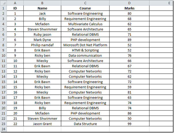
Now we will add new column Grade, which will contain grades secured by the students. Now for this, we will be using VLOOKUP function for looking up values from other table that contains sample data for grades.
Create two new columns containing marks range (sorted in any order) and corresponding grades. you don’t need to create them in a new worksheet, you can place anywhere in the existing datasheet as we just want to get values from it.
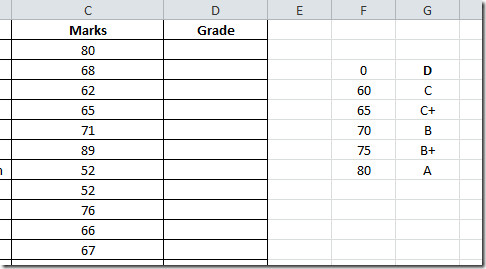
Now in the Grade first row, we will write VLOOKUP function. The syntax of this function is
VLOOKUP(lookup_value, table_array, col_index_num, [range_lookup] )
The first parameter of the formula lookup_value defines the value of the number which we will be looking in the newly created table. We need to lookup the value 80 (Marks field) in the newly created table. The next parameter, table_array defines the table we will be referring to in our case it will be newly created table, containing ranges of marks and grades. col_index_num defines data from which column we want to extract values to show, in our case it is the second column that contain grades range. [range_lookup] lets you to choose an option either TRUE(approximately matching of values) or FALSE (Exact matching of values).
We will write this function in Grade first row, it will go like this;
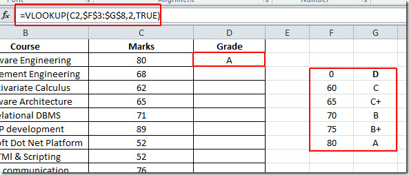
=VLOOKUP(C2,$F$3:$G$8,2,TRUE)
In the formula parameters, C2 is cell of column Marks which contain marks secured by students, F3:G8 is the location of the newly created table, containing ranges of marks and grades (use absolute referencing with $ sign), 2 in the formula means that values from second column will appear, and TRUE defines that we need approximately match as we have included ranges not exact values.
After evaluating formula, it will show grade A in Grade column as shown in the screen shot below.
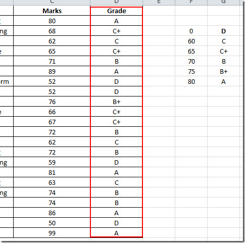
Now apply this function over the whole Grade column, drag the plus sign towards the end of Grade column to apply it over, as show in the screen shot below.
Now we also want to calculate the prize money for each student. for instance, we assume the following criteria.
For grade A $1000
For grade B+ $700
For grade B &600
For grade C+ $250
For grade D N/A
The criteria defined contains the exact value, so we will be making a small change in the parameters of the function. we will be choosing FALSE from [range_lookup] instead of TRUE as we want to show the exact match.
D2 contains the grade secured by students, so it will check the value in Grade column against the newly created columns, containing prize money criteria, as shown in the screenshot below.
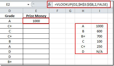
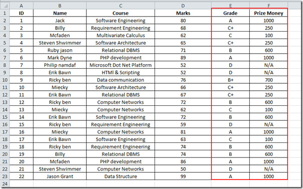
Now apply the function in Prize Money column to view the prize money won by each student. Now as you can see in the screenshot below that by using VLOOKUP function it is easier to look up specific values for populating new fields by connecting different columns.
You can also check out our previously reviewed guides on How to embed videos in Excel 2010 & Adding Outlook email tool in Excel.

Does the table array have to be part of the worksheet as a separate tab or can it be located outside the worksheet? If so, what’s the syntax?
Hi all,
if any one have solution of below given table please tell me.
Code
Stock
FCH/BS/00040
(DESSERT SERVERS)
8 SET
Delhi-NCR
2 SET
Gurgaon-HR
3 SET
Mumbai-MB
3 SET
FCH/BS/00358
(MAMBOO SPUN ORBIT WALL ART D100)
8 PCS
Delhi-NCR
1 PCS
Gurgaon-HR
2 PCS
Mumbai-MB
1 PCS
Chennai-CHN
2 PCS
Bangalore-BLR
2 PCS
FCH/BS/00410-T4
(JIN ,T4 GRAPHIC PATTERN ,5X12INCH)
12 PCS
Chennai-CHN
12 PCS
FCH/BS/00410
(TAMA ,BLACK COLOUR 5X12INCH)
23 PCS
Gurgaon-HR
6 PCS
Mumbai-MB
9 PCS
Chennai-CHN
4 PCS
Delhi-NCR
4 PCS
FCH/BS/00412-T11
(MARKO T11 GRAPHICS PATTERN 6X14INCH)
18 PCS
Mumbai-MB
6 PCS
Chennai-CHN
4 PCS
Delhi-NCR
8 PCS
FCH/BS/00413-T10
(HOSHI,T10 GRAPHIC PATTERN 6.5X9INCH)
6 PCS
Chennai-CHN
2 PCS
Delhi-NCR
4 PCS
Code
Stock
Delhi-NCR
Gurgaon-HR
Mumbai-MB
Chennai-CHN
Bangalore-BLR
FCH/BS/00040
(DESSERT SERVERS)
8 SET
FCH/BS/00358
(MAMBOO SPUN ORBIT WALL ART D100)
8 SET
FCH/BS/00410-T4
(JIN ,T4 GRAPHIC PATTERN ,5X12INCH)
12 SET
FCH/BS/00410
(TAMA ,BLACK COLOUR 5X12INCH)
23 SET
FCH/BS/00412-T11
(MARKO T11 GRAPHICS PATTERN 6X14INCH)
18 SET
FCH/BS/00413-T10
(HOSHI,T10 GRAPHIC PATTERN 6.5X9INCH)
6 SET
thanks & best regards,
Sajjan Singh
Hi, Im unable to use VLOOKUP formula in excel 2010 for a particular data…
pls help..
It is very helpful. Thank you.
superb explanation
thank you very much it was very useful
ffffffffffffff
ffffffffffffffffffffffff
ffffffffffffffffffffffffffff
ffffffffffffffffffffffffffffff
e
fffffffffffffff
helol
Hey big boyz, anyone else think Luke Miller is fit
stop commenting as meee
Really stupid!
GAYYBOOYS
Stupid
you smell like dog buns, UNACCEPTABLE!!!!!! :{
This tutorial was very helpful…..Learned alot
nice example
thanks, this as really been helpfull.
i have been trying to use the function but every time it is giving me value for data at the end of the cloumn not the exact data it is kind of weird i dont know how to solve this any suggestion please
Thanks,i got a idea now. how to use lockup function in excel.
Thanks for sharing the useful information with example.
Did I miss it, or did you forget to mention the BIG qualifier for the function to work: The lookup table lookup column MUST have the numeric or alpha data in rows of ascending order or it won’t work.
How to you return a zero instead of the #N/A?
PLEASE,
EXPLAIN ABOUT TRUE,FALSE IN VLLOKUP
It’s also useful thing Now And Future am i right guy’s ?
When using Vlookup with numerical data, as currently coded it does not return the nearest value in the lookup table, only the highest value exceeded. Would it be so difficult to incorporate such a capability? I think there are many out there who want to use it that way.
very well explained!! Thnx.
Thank you, it was very usefull to me. GRACIAS.
great thanks
what if I want to multiply my Look-up value by the table array. I know I can write a formula to obtain my answer, but if I could create a table that I can reuse over & over…..
so, per your example, what if the prize money was a % and not a fixed amount?
SINCE it is a small table it is understandable and we are creating another table with comparable figures. But whereas in case of Banking sector, MNC where 1000 of records of maintained with different values, nos. names, how is it possible to create comparing table, without which the formula serves no purpose. is there any way that u can explain from a to z.
Mythili
Thanks it is very useful
romel
Thank you very much shalini
its very use full for me
Very nyc but want more too learn
it is very useful
Rahul Dancer
An excellent article about how to use vlookup, it is very useful and easy to understand. Thanks!!!
It is really very useful for, who ones wants to learn how to use formulas in Excel speardseets. Thanking for such great helpful ideas. continue…
it is very useful
shalini
Hai shalini if you have any other idea for excel formulas tell me.
what is use of vlookup function in excel
i am trying to use from morming but i dont no how it will effect