Excel Database Functions: DAVERAGE and DSUM
Excel 2010 enables user to create database table for performing database functions and applying formulas. Excel 2010 inherited different database functions which lets one tweak data from the specified database, you just need to choose the primary field, and apply a certain condition for pulling out specified content from database. THE DAVERAGE and DSUM functions are used to find out the average and sum of the database values as specified in criteria.
Launch Excel 2010 and open a spreadsheet on which you want to apply database functions; DAVERAGE, and DSUM. For illustration, we have included database table containing fields; Name, Course, Marks, Grade, and Status.
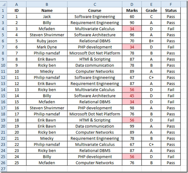
In this table we have 10 students in total who studied different courses. We will be finding out the average & sum of marks secured by the students excluding the marks less than 59. For this, first we will be creating a Criteria table and then other labels where we are going to show the resultant value in the same spreadsheet, as shown in the screenshot below. The labels in the Criteria table must be same as in database table i.e Name and Marks.
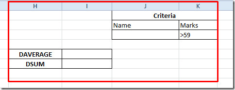
Now for find out out average of all the students who have secured marks greater than 59, we will use DAVERAGE function.
The syntax of DAVERAGE function is;
=DAVERAGE(database,field,criteria)
The database in the argument refers to the location of the table which will be considered as database, the second argument field refers to the number of field/column in which we have defined criteria and the last argument refers to the criteria defined either directly or location of table where it is defined.
We will be writing this function as;
=DAVERAGE(B1:F26,3,J2:K3)
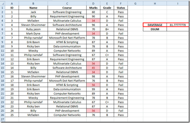
B1:F26 in the function as argument refers to the location of database table, 3 is the number of field/column in the database table (from Name, Course, and Marks) as we are checking values in Marks table for meeting defined criteria, and the last argument is J2:K3 which refers to the criteria table. It will yield average of the marks (greater than 59 secured by the students), as shown in the screenshot below.
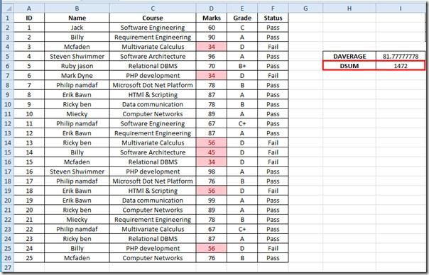
Now for finding out the sum of marks through DSUM function. The syntax is exactly same except the name of the function would change to DSUM. We will write this function as;
=DSUM(B1:F26,3,J2:K3)
It will yield the sum of all the students who have passed the courses (secured marks greater than 59).
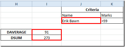
Now if you want to find out the average and sum of specific student, just enter the student’s name in the Criteria table and it will immediately show the corresponding results.
You can also check out previously reviewed Excel function; DCOUNT, ISTEXT, ISNUMBER, Logical Functions, INFO, SUMSQ, DOLLAR, SUMPRODUCT, SUMIF, COUNTIF, VLOOKUP, HLOOKUP ,PMT, and LEN.
